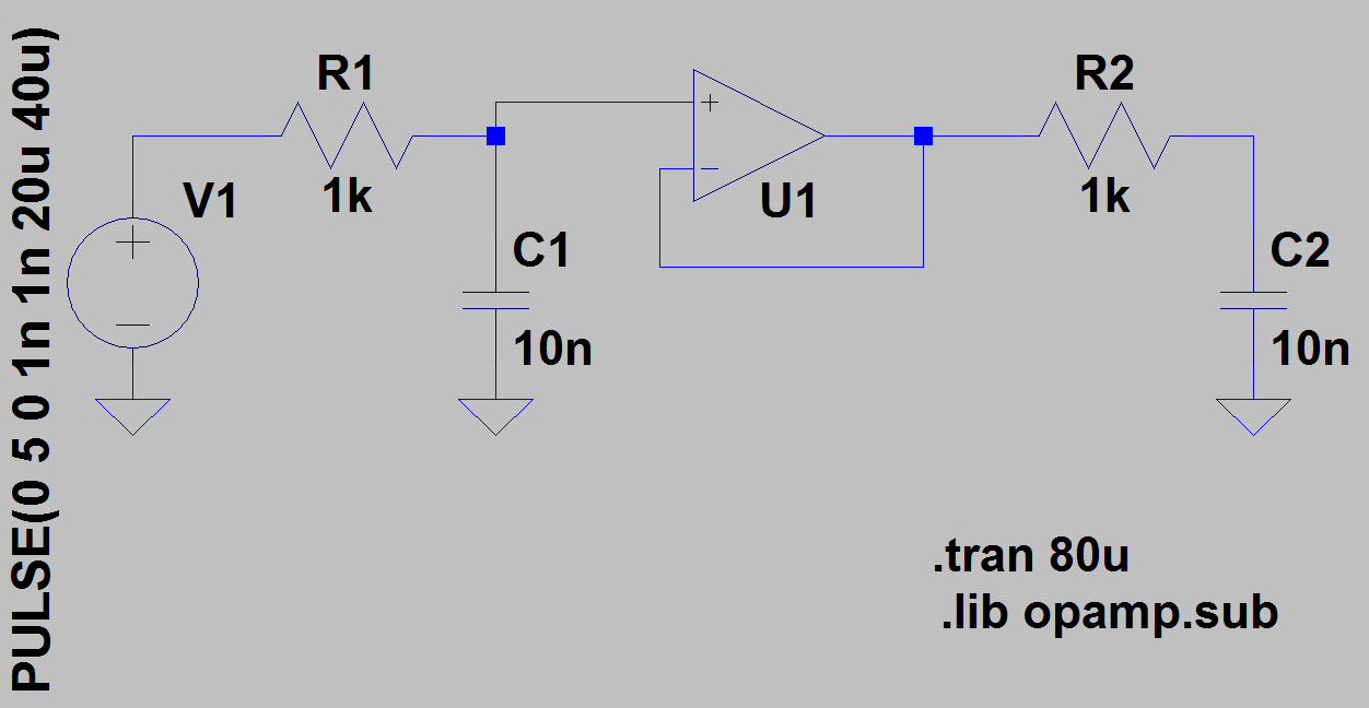
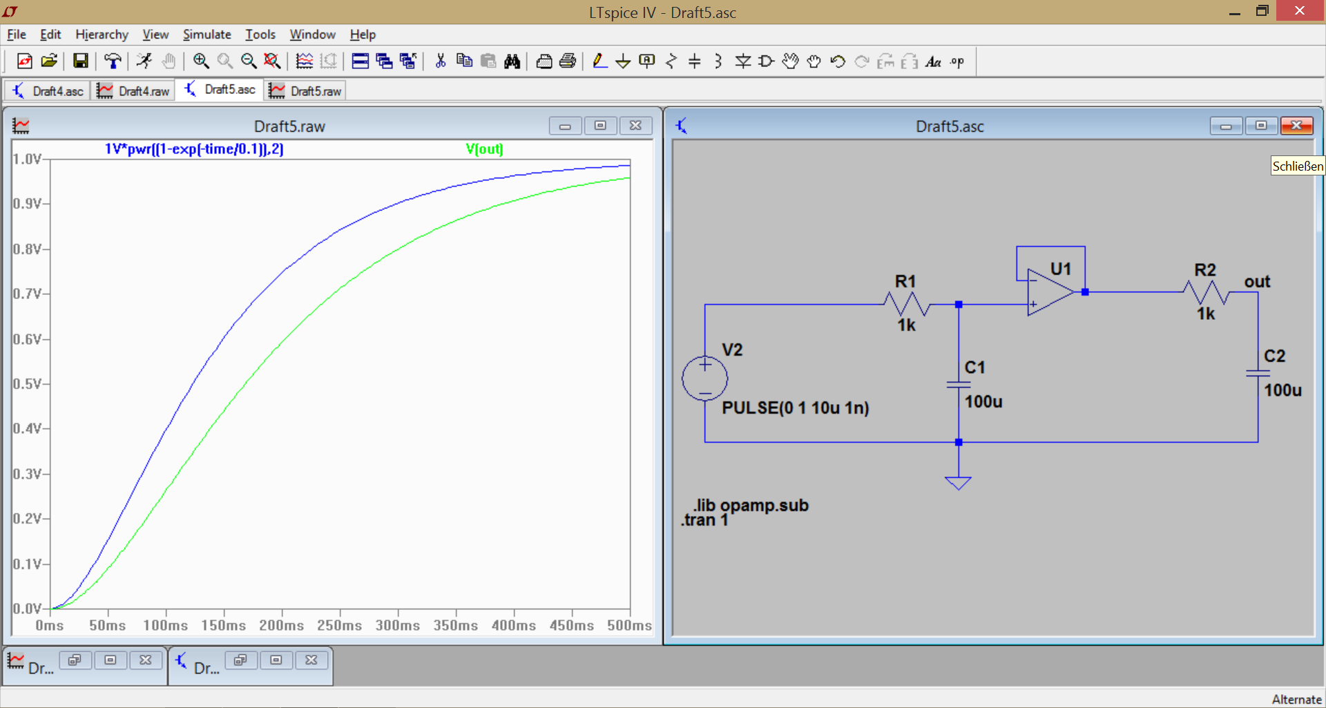
Hallo zusammen,

angenommen, ich habe zwei RC-Glieder hintereinander, die durch einen OPV
getrennt sind und sich deshalb nicht gegenseitig beeinflussen. Siehe
Schaltung im Anhang.

Die Ladespannung am ersten Kondensator C1 berechnet sich dann zu:
Jetzt möchte ich gerne zu einem beliebigen Zeitpunkt t die Ladespannung
am hinteren Kondensator C2 ausrechnen. Ich knobel schon eine ganze
Weile, aber komme nicht darauf.

Weiß jemand Rat und kann mir helfen?

Werner
Mit "Ladespannung" meinst Du vermutlich die Sprungantwort des ersten
RC-Gliedes (da die Gleichspannung am Eingang bei der TRAN-Analyse zum
Zeitpunkt t=0 praktisch eingeschaltet wird.)
Daraus ergibt sich dann durch die Integration des Ladestromes die
e-Funktion des ersten Teils (die Du ohne Integration gleich angenommen
hast).
Beim zweiten RC-Glied hast Du nun keinen Eingangssprung mehr - also
musst Du auf die Definition (Zusammenhang Uc und Ic) zurückgreifen und
damit den Spannungsumlauf formulieren:
Uc=(1/C)*[Integral Icdt], oder in der Form
Ic=C*dUc/dt.
Hallo,

Google mal zu Sprungantwort PT1 und PT2 Glied. Da findet sich vieles.
Ansonsten Buch zu theoretische Elektrotechnik oder Regelungstechnik
konsultieren.

Mfg
Was ist daran so schwer?

die Spannung an einem Kondensator ist:
Uc(t) = U0*(1-exp(t/tau)

An deinem zweiten RC-Glied liegt die Spannung nicht sprunghaft an,
sondern steigt mit der des ersten RC-Glieds:

Uc2(t) = Uc1(t)*(1-exp(t/tau)

Bei unterschiedlichen R und C berechnet sich die Spannung zu einem
beliebigen Zeitpunkt folglich:

Uc2(t) = U0 *(1-exp(t/tau1)*(1-exp(t/tau2)

Bei identischen R und C vereinfacht es sich zu:

Uc2(t) = U0 *(1-exp(t/tau)²

Wenn dein U0 Zeitabhängig ist musst du das entsprechend anpassen. Und
deine Startspannung ist auch relativ unproblematisch einzubauen.
Kevin M. schrieb:> Was ist daran so schwer?>> Uc2(t) = U0 *(1-exp(t/tau1)*(1-exp(t/tau2)
Durch diesen Ansatz setzt Du voraus, dass das 2. RC-Glied ebenfalls als
Eingang einen Sprung erhält, was aber - auch Deinen eigenen Worten nach
- nicht der Fall ist. Damit widersprichst Du Dir selber und das Ergebnis
kann nicht einfach das Produkt zweier Sprungantworten sein.
Werner schrieb:> Jetzt möchte ich gerne zu einem beliebigen Zeitpunkt t die Ladespannung> am hinteren Kondensator C2 ausrechnen.
Brauchst du eine geschlossene Formel oder reicht die die Ladekurve?
Werner schrieb:> Ich glaube, der Hinweis mit der Sprungantwort des PT2 Glieds ist eine> heiße Spur.
Ja, aber man muss drauf achten, dass beide Pole reell sind - also die
Polgüte dieser Tiefpass-Anordnung zweiten Grades gleich oder kleiner als
0,5 ist.
Lutz V. schrieb:> Ja, aber man muss drauf achten, dass beide Pole reell sind
Das wird sich bei einfacher Serienschaltung von Tiefpässen 1.Ordnung
nicht vermeiden lassen.
Lutz V. schrieb:> Durch diesen Ansatz setzt Du voraus, dass das 2. RC-Glied ebenfalls als> Eingang einen Sprung erhält, was aber - auch Deinen eigenen Worten nach> - nicht der Fall ist.
Nein mach ich nicht, da die Spannung am zweiten eben mit der des ersten
ansteigt. Oder was soll das sonst sein wenn ich schreibe:
Uc2(t) = Uc1(t)*(1-exp(t/tau)
wohl kaum ein Sprung....
Wenn du mir nicht glaubst schau dir die Bilder im Anhang an...
Wolfgang schrieb:> Lutz V. schrieb:>> Ja, aber man muss drauf achten, dass beide Pole reell sind>> Das wird sich bei einfacher Serienschaltung von Tiefpässen 1.Ordnung> nicht vermeiden lassen.
Mein Kommentar bezog sich auf das erwähnte PT2-Element. Und da gibt es
sogar relativ häufig ein komplexes Polpaar.
Kevin M. schrieb:> Nein mach ich nicht, da die Spannung am zweiten eben mit der des ersten> ansteigt.
Aber Dein Ergebnis besteht doch aus dem Produkt zweier Sprungantworten
(1-exp)*(1-exp).....Also machst Du es doch!
Was zeigen denn Deine Bilder? Eine Sprungantwort 1. Ordnung und eine 2.
Ordnung. Ja - und? Wo ist denn der Beweis, dass es dabei um das PRODUKT
zweier Sprungantworten geht?
Dazu musst Du zwei Sprungantworten 1. Ornung erzeugen und die dann zum
Schluss multiplizieren! Und dann vergleichen...
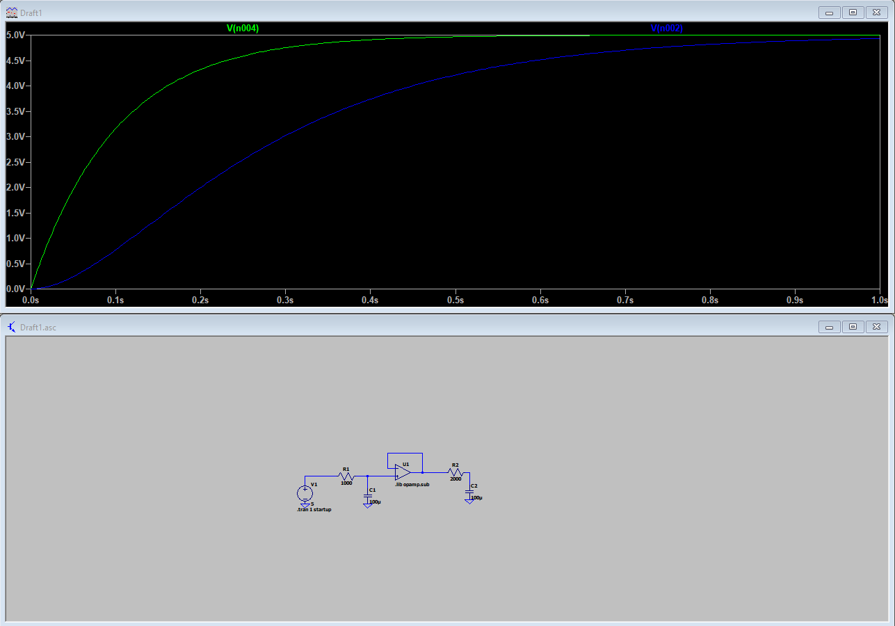
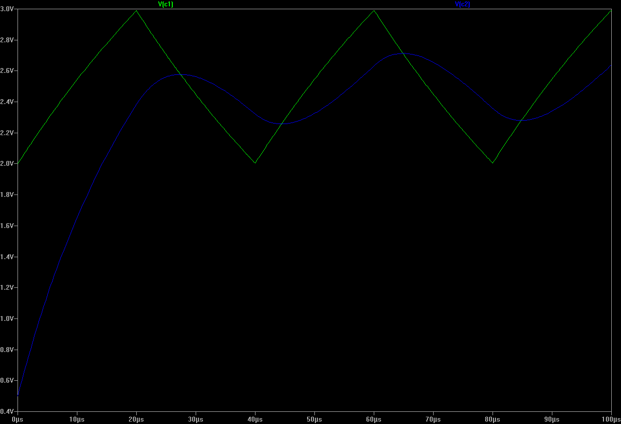
H. B. schrieb:> Miss mit Spice mal den Spannungsverlauf an C2 im Verhältnis zu C1.> Daraus kann man schon mal Rückschlüsse auf das Verhalten ziehen.
Den Kurvenverlauf habe ich hier angehängt. Grün ist die Spannung an C1
(Formel bekannt), blau ist die Spannung C2 (Formel gesucht).
Wolfgang schrieb:> Brauchst du eine geschlossene Formel oder reicht die die Ladekurve?
Ich hoffe, ich habe Deine Frage richtig verstanden: Ich möchte die
Ladekurve U_C2(t) für beliebige t berechnen. Die Entladekurve brauche
ich nicht.
Lutz V. schrieb:> Ja, aber man muss drauf achten, dass beide Pole reell sind - also die> Polgüte dieser Tiefpass-Anordnung zweiten Grades gleich oder kleiner als> 0,5 ist.
Ich habe den Eindruck, für meine Frage muss ich mich in die Berechnung
von Filtern einarbeiten. Ich habe heute Vormittag mit der Formel
herumgespielt:
Für tau_1 = tau_2, wie es in meinem Beispiel ist, werden die hinteren
Terme zu unendlich. Das ist natürlich ungünstig. Sind das die "Pole",
von denen ihr sprecht?
Lutz V. schrieb:> Aber Dein Ergebnis besteht doch aus dem Produkt zweier Sprungantworten> (1-exp)*(1-exp).....Also machst Du es doch!
Wie du meinst, es ging darum die Spannung zu berechnen das habe ich
gemacht. Ich hab es schon vor langem aufgegeben mit den viel schlaueren
Menschen hier zu diskutieren.
Lutz V. schrieb:> Dazu musst Du zwei Sprungantworten 1. Ornung erzeugen und die dann zum> Schluss multiplizieren! Und dann vergleichen...
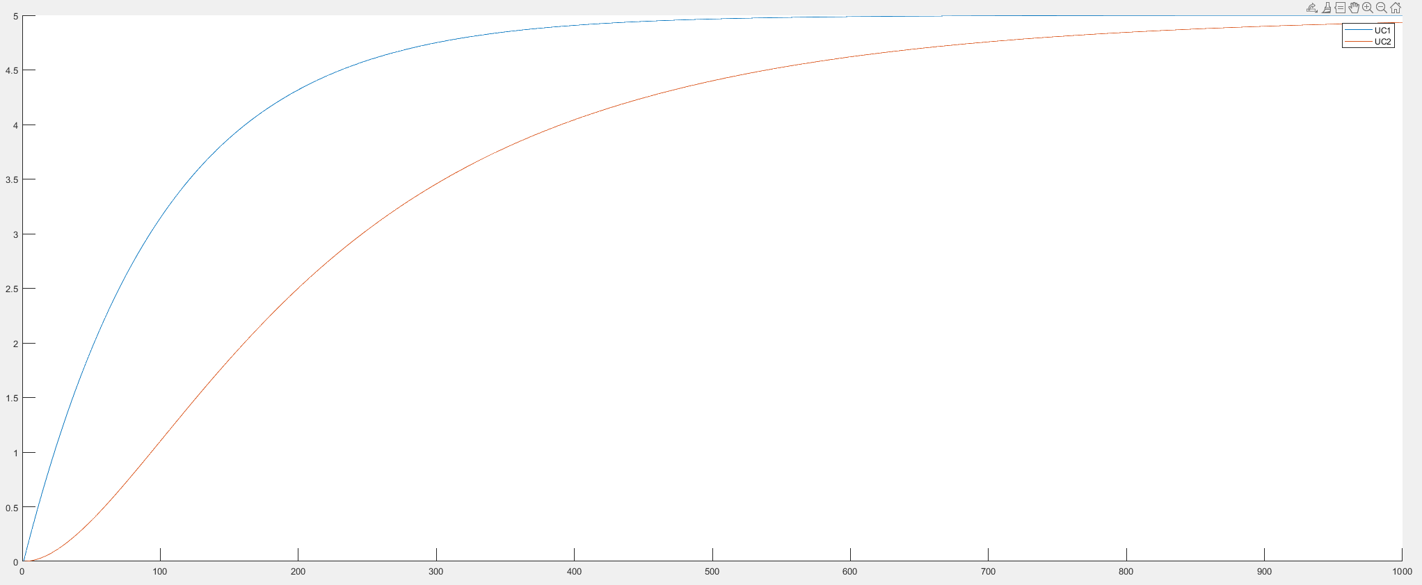
Was glaubst du womit ich die Matlab Figure erzeugt habe? in Paint
gemalt? Wohl kaum :D
Kevin M. schrieb:> Wie du meinst, es ging darum die Spannung zu berechnen das habe ich> gemacht
aber dein Ergebnis stimmt halt leider nicht. Im Anhang mal der direkte
Vergleich deiner Formel mit dem simulierten Verlauf. Die Kurven sehen
sich zwar ähnlich, aber direkt nebeneinander aufgetragen wird der
Unterschied schon deutlich, oder?
Kevin M. schrieb:> Wenn du mir nicht glaubst schau dir die Bilder im Anhang an...
wenn man ein bisschen genauer hinschaut sieht man den Unterschied
zwischen deiner Berechnung und der Simulation auch schon in deinen
Bildern. Vergleiche z.B. mal, wann bei deinen Bildern jeweils 1V am
zweiten Kondensator erreicht wird.
Aua was ist denn hier los? Die beiden PT1 Übertragungsfunktionen werden
im Frequenzbereich multipliziert, nicht im Zeitbereich. Im Zeitbereich
sind das alles Differentialgleichungen (Funktionen von t und deren
Ableitungen nach t), da kannst du nicht einfach für U eine zeitabhängige
Funktion in die Lösung der DGL einsetzen, da diese dann nicht mehr die
Lösung ist...
Achim S. schrieb:> aber dein Ergebnis stimmt halt leider nicht.
Hast du die fehlende Übertragungsfunktion des Opamps bedacht? Die ist in
LTSpice nicht ideal...
Kevin M. schrieb:> Was glaubst du womit ich die Matlab Figure erzeugt habe? in Paint> gemalt? Wohl kaum :D
Das von Dir beigefügte Schaltbild hat aber was ganz anderes
gezeigt....eine eigentümliche "Beweisführung".
Kevin M. schrieb:> Ich hab es schon vor langem aufgegeben mit den viel schlaueren> Menschen hier zu diskutieren.
Gute Entscheidung.....lies Dir mal dieAntwort von Achim S. durch....
Kevin M. schrieb:> Hast du die fehlende Übertragungsfunktion des Opamps bedacht? Die ist in> LTSpice nicht ideal...
die spielt bei den gewählten Zeitkonstanten so überhaupt gar keine
Rolle...
Kannst ja mal die Parameter des OPV in der Simu um eine Größenordnung
verbessern und schauen, wie riesig der Einfluss auf die Kurvenform ist.
Jetzt habe ich noch das Problem, dass die Kondensatoren zu Beginn auf
eine Startspannung geladen sein sollen. Bei identischen Spannungen ist
es leicht. Aber bei unterschiedlichen Spannungen probiere ich es jetzt
eine Weile, aber der Groschen fällt einfach nicht.

Kann mir nochmal bitte jemand helfen?
Kevin M. schrieb:> Hast du die fehlende Übertragungsfunktion des Opamps bedacht? Die ist in> LTSpice nicht ideal...
Das Ding läuft als Spannungsfolger. Zeig mal, welchen Unterschied du da
in dieser Schaltung im Vergleich zum idealen OP siehst.
Was meinst du wohl, welchen Einfluss die Übertragungsfunktion des OP auf
die Übertragungsfunktion des Spannungsfolgers in dem relevanten
Frequenzbereich hat?
Funktioniert folgender Ansatz?

Formel (gilt für τ1 != τ2):
Erweiterung um Faktoren x1 und x2, die die Startspannung der
Kondensatoren U_Start1 und U_Start2 abbilden sollen:
Festlegung bekannter Werte für x1 und x2:

(1) Folgendes muss für x1 und x2 gelten, damit bei bereits voll
geladenem C1 die Formel für die Sprungantwort am zweiten RC-Glied
erscheint:
(2) Das Gleiche aus (1) gilt analog für C2 / das erste RC-Glied:
(3) Per Simulation kann ich sehen, dass folgendes gilt, wenn beide
Startspannungen identisch sind:
Als nächstes müsste ich jetzt eine Formel für x1 und x2 entwickeln, die
die eben genannten Bedingungen erfüllt. (Sofern das eben alles richtig
war, natürlich.) Das heißt, sie müsste folgendes abbilden:
Die Spannung U_unendlich ist die zeitlich konstante Spannung der Quelle
ganz links im Schaltbild. x0 und y0 sind die (dimensionslosen)
Ladespannungen der Kondensatoren zum Zeitpunkt t = 0.

Für die Funktion f(t) ist eine Fallunterscheidung nötig. Im Fall alpha
ungleich beta ist
zu setzen, im Fall alpha = beta dagegen
Wenn Du die Probe machst, wirst Du sehen, dass die angegebenen Lösungen
tatsächlich die Differentialgleichungen
beziehungsweise
erfüllen. Die Herleitung dieser DGs sollte klar sein (Addition der
Spannungen am Widerstand und Kondensator unter Verwendung von U = RI und
I = dQ/dt und Q = CU).

Die Standardmethode für den Problemtyp "inhomogene, lineare DG erster
Ordnung mit konstanten Koeffizienten" ist die sogenannte "Variation der
Konstanten". Kannst Dich ja schlaumachen und es dann selbst probieren.
Ansonsten benötigst Du nur Stift, Papier (zwei DIN A4-Seiten für die
Lösung der y-DG) und die Stammfunktion von e^x.

>Was haltet ihr davon?

Wenn Du solche Feinheiten wie z. B. die sich hier ergebende
Fallunterscheidung korrekt ausknobeln kannst, bist Du gut.
Chapeau! Deine Formel funktioniert einwandfrei. Beeindruckend, wie Du
mit Formeln umgehen kannst!

Ich wollte die Lösung unbedingt wissen und habe erst eine Weile mit
Ausprobieren verbracht. Seit gestern Abend lese ich mich nun in DGL ein
und glaube, das ein oder andere auch verstanden zu haben. Trotzdem
probiere, rechne und knobel ich herum, ohne auf die Lösung zu kommen.

Vielen Dank, dass Du Dir die Zeit für eine Antwort genommen hast! Danke
natürlich auch an alle anderen, die mir weiter geholfen haben! Das war
sehr nett!

Werner
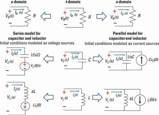
Dump the Laplace transform, it's too much hassle and too much knowledge
required. Use Heaviside's transform!

The voltage source that switches from Vs to Vz at t=0 may be represented
as a series connection of two voltage sources. One switches off from Vs
to zero, the other switches on from zero to Vz. If the unit step is
denoted as u(t), the voltage applied to the input is:
The transfer function from the input voltage Vi(t) to the output voltage
Vo(t) on the second capacitor assuming R1=R2 and C1=C2 is
It's calculated by whatever means, ranging from manually applying the
Ohm's law to employing a symbolic solver.
Now Vi(t) has to be transformed through F(p). For constant DC term the
transform is F(0). For the unit step term, the transform is found using
the Carson-Heaviside transform table (or Laplace's, but multiply the
table by operator 's', so that transform of unit step equals one).
This expression is valid for all t from minus to plus infinity, unlike
the Laplace transform, which starts from t=0.
Heaviside transform requires only high-school math and the knowledge of
Euler's formula. Also, one doesn't struggle with initial conditions,
since they are calculated automatically in the process.

P.S. Sorry for potential violation of forum rules, but my German is even
worse than my English.
Bin sehr beeindruckt über die gekonnten Herleitungen über
Übertragungsfunktion und Differenzialgleichungen. Ich würde allerdings
alles viel simpler betrachten.  Beide TP sind über einen Buffer
entkoppelt, sodass der Ausgang des ersten der Eingang des zweiten ist.
Ich nehme nun das Bodediagramm des ersten TP und bekomme irgendwo meinen
-3dB-Punkt und idealerweise danach einen Spannungsabfall von 6dB pro
Oktave. Da beide TP gleich dimensioniert sind (und entkoppelt) sieht der
zweite im Durchlassbereich bis zum 3dB-Punkt die 0-dB des ersten und
gibt sie auch aus. Danach sieht der zweite die -6dB pro Oktave, die er
seinerseits um  6dB abschwächt und am Ausgang stellen sich -12dB pro
Oktave ein. Das alles hätte man in Spice im Nu dargestellt...ich wollte
es aber "zu Fuß" haben...
Gruß Rainer
LumpedNetwork schrieb:> Dump the Laplace transform, it's too much hassle and too much knowledge> required. Use Heaviside's transform!
That's a neat approach! But to be honest, I was far away from using such
tricks as I was still struggling to understand the task itself. So
thanks for your hint.
There is one drawback with your solution though: I'd like to set the
initial voltage for both capacitors. However with your formular it's
possible to set the source voltage only.
Rainer V. schrieb:> Ich nehme nun das Bodediagramm des ersten TP und bekomme irgendwo meinen> -3dB-Punkt und idealerweise danach einen Spannungsabfall von 6dB pro> Oktave.
Das hatte ich auch probiert. Aber damit funktioniert es nur im
Frequenzbereich. Ich suche dagegen das Verhalten im Zeitbereich.
@ LostInMusic und alle anderen : Hast Du / habt ihr noch einen Tipp,
wie ich die Formel nach t umstellen kann? Ich wüsste gerne, nach welcher
Zeit t eine bestimmte Spannung am Ausgang (= Kondensator C2) erreicht
ist.
Ich lande bei meinen Versuchen nach Substituieren immer bei einer
Gleichung der Form:
Diese Form ist, wenn ich es richtig sehe, nicht nach t umstellbar. Oder
doch? Gibt es da einen Trick?
Werner schrieb:> There is one drawback with your solution though: I'd like to set the> initial voltage for both capacitors. However with your formular it's> possible to set the source voltage only.
It's a feature of Heaviside transform, not a bug. You can't set initial
conditions on BOTH voltage source AND capacitors. Because everything up
to t=0 is DC steady state, the voltage source has an infinite amount of
time to override any initial charge on these capacitors.
If someone is dead set on having a particular voltage on the capacitors
at t=0, he may use a unit step voltage source in series with a capacitor
to add some voltage. Alternatively, a parallel-connected current source
that injects some charge with a Dirac impulse can be used. Now, if the
source is also a unit step, we're back at Laplace transform, actually.
> Diese Form ist, wenn ich es richtig sehe, nicht nach t umstellbar.https://math.stackexchange.com/questions/129504/solving-a-sum-of-exponentials
LumpedNetwork schrieb:> If someone is dead set on having a particular voltage on the capacitors> at t=0, he may use a unit step voltage source in series with a capacitor> to add some voltage. Alternatively, a parallel-connected current source> that injects some charge with a Dirac impulse can be used.
I must admit that I don't have the skills to understand how to do that.
I hope this will be helpful to the others.
LumpedNetwork schrieb:>> Diese Form ist, wenn ich es richtig sehe, nicht nach t umstellbar.>> https://math.stackexchange.com/questions/129504/solving-a-sum-of-exponentials
In the link they're telling that there is a solution for exponents
smaller than 5. Which would be fine as I can scale my exponent without
restrictions. That is, I can increase 𝜏 such that the exponent becomes <
5, if I also increase t accordingly. Right?
Werner schrieb:> In the link they're telling that there is a solution for exponents> smaller than 5. Which would be fine as I can scale my exponent without> restrictions. That is, I can increase 𝜏 such that the exponent becomes> < 5, if I also increase t accordingly. Right?
No, what they mean is that with substitution
this equation can be rewritten as
And this kind of equation is solvable only for integer ratio tau1/tau2
no higher that 4.
> I must admit that I don't have the skills to understand how to do that.> I hope this will be helpful to the others.
OK. When the student is ready, the teacher will appear :)
It's a well-known technique in Laplace transform. It allows inserting
initial conditions into the circuit by connecting artificial sources to
reactive elements.
Does that mean that for any given PT2 element with tau1/tau2 > 5, it is
impossible to calculate the time after which a specific output level
is reached?!
Gruss

Ich finde den Ansatz von Kevin M. am
30.1 um 4:34 konventionell für richtig.
Auch wenn das Binom durch einen Tippfehler
unter geht.
Mit Tau1 und Tau2 in e, entsp. b1 u. b2.
1^2 -b2 -b1 + b1*b2.
Das lässt sich darstellen.
Der Rest hin zu t ist höhere Mathematik.
Die Gegenständliche Darstellung lässt sich variieren, Variation der
Parameter bz. Konstanten, sind dann Analytisch ( Kurvendiskusion )
zugänglich.

Dirk St
Werner schrieb:> Does that mean that for any given PT2 element with tau1/tau2 > 5,> it is> impossible to calculate the time after which a specific output level> is reached?!
To be able to solve this equation algebraically, the ratio of tau1/tau2
should be an integer 1, 2, 3, or 4. But nothing rules out the numerical
solution for any other ratio. SPICE does it, after all.
Usually, this is not a problem. When time constants tau1 and tau2 differ
by a large amount (poles are well split), only one constant dominates
because for LPF and HPF response the exponents are scaled with these
time constants. Beware, that no scaling happens for BPF. One can deduce
that from the Laplace transform table.
Werner schrieb:> Ich suche dagegen das Verhalten im Zeitbereich.
dann mache ich es noch mal intuitiv. Beide Kondensatoren sind entladen
und es wird eine Spannung Ui an den ersten Widerstand angelegt. Dann
steigt die Spannung an C1 nach der "tau-Formel". D.h. u.a. Spannung an
C1 ist nach 5 tau (oder auch x tau) ~Ui. Diese Spannung sieht nun R2 und
läd C2 nach der selben tau-Formel auf (R1=R2, C1=C2). Damit erwarte ich,
dass die Spannung an C2 hinter C1 herhinkt, bis sie sich dann bei ~Ui
treffen. Und damit ergibt sich für mich die Frage, warum in den früheren
Ansätzen mit zwei verschiedenen tau gerechnet wird. Die DG ist doch nur
deshalb nicht allgemein lösbar. Vielleicht bin ich aber auch auf dem
Holzweg...
Gruß Rainer
>Diese Form ist, wenn ich es richtig sehe, nicht nach t umstellbar. Oder>doch? Gibt es da einen Trick?
Es gibt leider keine Möglichkeit, die Gleichung
a = e^(−t/τ2) + e^(−t/τ1)
nach t aufzulösen (von wenigen Sonderfällen abgesehen). Der Trick, das
als
a = x + x^(τ1/τ2)
umzuinterpretieren und dann z. B. für τ1/τ2 = 2 oder 3 oder 4 die
Nullstelle des entsprechenden Polynoms analytisch zu berechnen, könnte
natürlich funktionieren. Ob das dann aber für Deine Anwendung zu einer
zufriedenstellenden Lösung führt, hängt sicher auch von der speziellen
Aufgabe ab, die diese Schaltung erfüllen soll. Angenommen, Du legst Dich
auf τ1/τ2 = 3 fest: Wie genau kannst Du die "3" erreichen? Die Werte von
R1, R2, C1 und C2 unterliegen ja immer gewissen Schwankungen z. B. durch
Temperatur, Alterung usw. Das führt dann nur zu einer weiteren Frage:
Welches Vertrauen kannst Du noch in Dein berechnetes Ergebnis haben,
wenn die 3 mal ein bisschen größer oder kleiner ist? Ehrlich gesagt: Ich
hätte da eher kein gutes Gefühl. Da würde ich dann lieber nach einer
Ersatzschaltung suchen, die denselben Zweck erfüllen kann, aber
einfacher zu berechnen ist.
I understand, we've reached the point where different initial conditions
are being investigated, but I'd like to go one step back to show how to
develop the solution with initial conditions = 0 in the frequency domain
instead of in the time domain.

From a system theoretical perspective, a RC circuit is a PT1 element
with known (look it up in tables) transfer function
, where H is the transfer function ("Übertragungsfunktion"), Y the
Laplace transformed output (aka the voltage across the capacitor) and U
the input to the circuit (laplace transformed, too).

Now here is the trick. Since you use a buffer to decouple the second RC
element from the first one, there is no feedback from the second to the
first one, they are independent. Therefore you can multiply the two
transfer functions to get the system's overall answer:
The tricky part is to figure out the U which is the laplace transformed
input signal (V1 voltage). Luckily it's easy here, it's an input step
function (called Heaviside function) from 0 to a fixed value. Its
Laplace transform is 1/s (or K/s for a constant gain) see
https://de.wikipedia.org/wiki/Laplace-Transformation#Korrespondenztabelle.

Apply it and transform it back to time domain. This can be done via
partial fraction decomposition (which is indeed a bit complicated, but
still basic math, no fancy stuff, see
https://de.wikipedia.org/wiki/Partialbruchzerlegung. You can also use
WolframAlpha to calculate it ;)

With tau1 = R1C1 and tau2 = R2C2:
Transform it back (simply using tables, no calculation)
Θ(t) is the Heaviside function that equals 1 for t>0. K is a constant
factor, i.e. instead of an input voltage of 1 (V) you can have K=10 or
so. The transfer function is usually unit less, but you can also choose
K=10 V to have Volts.

This is exactly the result shown above, but without any formula in the
time domain. No U=RI, no Q=CU, no Kirchoff's law. It's just a slightly
different approach, coming from the system theory :)

However, initial conditions != 0 are a bit tricky and honestly I don't
know any way without transforming it to state space representation.

Note, this really only works when the circuits are perfectly decoupled
which is not often the case for electric circuits :)
Rainer V. schrieb:> Bin sehr beeindruckt über die gekonnten Herleitungen über> Übertragungsfunktion und Differenzialgleichungen. Ich würde allerdings> alles viel simpler betrachten. Beide TP sind über einen Buffer> entkoppelt, sodass der Ausgang des ersten der Eingang des zweiten ist.> Ich nehme nun das Bodediagramm des ersten TP und bekomme irgendwo meinen> -3dB-Punkt und idealerweise danach einen Spannungsabfall von 6dB pro> Oktave. Da beide TP gleich dimensioniert sind (und entkoppelt) sieht der> zweite im Durchlassbereich bis zum 3dB-Punkt die 0-dB des ersten und> gibt sie auch aus. Danach sieht der zweite die -6dB pro Oktave, die er> seinerseits um 6dB abschwächt und am Ausgang stellen sich -12dB pro> Oktave ein. Das alles hätte man in Spice im Nu dargestellt...ich wollte> es aber "zu Fuß" haben...> Gruß Rainer
Das ist übrigens quasi das grafische Pendant zu dem Multiplizieren der
beiden Übertragungsfunktionen was ich im Post zuvor beschrieben habe.
Das Verschieben in Bode Plot entspricht einer Multiplikation (einer
Verkettung).
Can't edit my posts :/ there is an error in the equation above. When
going from the product to the sum, the factor K needs be factored out,
i.e. brackets are missing. The end result should be correct.
Jan K. schrieb:> However, initial conditions != 0 are a bit tricky and honestly I don't> know any way without transforming it to state space representation.
There's a treatise on transients, where a general five-step solution
process is laid out
(http://cest.nau.edu.ua/ukr/person/zelenkov/book/Transients.pdf page
62).
Probably, I'm dumb and can't get it, but it seems absolutely crazy to
me. So, instead, I'm using this book as a source of problems for
test-driving the Heaviside transform. Currently, I've solved 2/3 of the
examples from there (beware, there are a lot of typos in this book, some
of them are quite grave). Worked like a treat, never had to resort to
any knowledge from differential equations course or complex analysis.
Also didn't have to bother with initial conditions or commutation laws.
So I'm still in search of a problem, that can't be solved with Heaviside
transform.
Feel free to write if you have one. Until then, Heaviside transform for
the win! :)
LumpedNetwork schrieb:> There's a treatise on transients, where a general five-step solution> process is laid out> (http://cest.nau.edu.ua/ukr/person/zelenkov/book/Transients.pdf page> 62).
Cool, thanks! Will look into that.
Strangely Heaviside was not taught in our classes and I can't find much
literature. Do you have some?
Although I'm Electrical Engineer, I like to approach things from the
system theory view (control theory) since this simply is where I'm
better at ;)
That said, the above approach (with initial conditions = 0) is quite
easy and does not require any kind of higher mathematical magic stuff.
IMO it's straight forward when you know the transfer function of the two
building blocks (two RC elements in this case), which you can look up in
tables. Then just concatenate (series connection = multiplication,
parallel = addition, see
https://de.wikipedia.org/wiki/Signalflussplan#Signalflussalgebra) them,
transform the input voltage to frequency domain (it can be a jump, a
sawtooth or sine, or much more), again using tables. Multiply everything
and make partial fraction decomposition (using a CAS ;)). If you do it
by hand - there is still no magic, just rearranging terms and fraction
numbers (with variables ;)). This is no stuff a degree is needed for.
Back transformation is relatively easy using tables again.
And this is a concept, you can use the same approach, same steps
everytime :)
However I'm not arguing the same is not true for Heaviside, I just don't
know.
LumpedNetwork schrieb:> Usually, this is not a problem. When time constants tau1 and tau2 differ> by a large amount (poles are well split), only one constant dominates> because for LPF and HPF response the exponents are scaled with these> time constants.
All right. So above equation is not solveable for t. I need to get rid
of at least one RC element, so that an exp() term drops out. Therefore,
my only chance is to become more specific with my problem, hoping that
this will allow for a simplification. Right?
Let's assume tau1 >> tau2. Let's also assume f > 1/( 2 PI tau1). As
before I am interested in what time it takes for Uc2 to reach a certain
level.
I did a simulation of the above. At the given frequency Uc1
approximately appears as a triangular waveform. That is, my first RC
element might be substituted by an integrator. Right again?
Theoretically I could now use the Heaviside transform. I would look-up
the integrator and apply it. Easy. However I still use initial voltages
at C1 and C2. So in the end I can not use it. At least not in its simple
form. Correct?
But still - is my task solveable? Can I provide random values for Uc2
and calculate the time t?
LostInMusic schrieb:> Es gibt leider keine Möglichkeit, die Gleichung>> a = e^(−t/τ2) + e^(−t/τ1)>> nach t aufzulösen (von wenigen Sonderfällen abgesehen).
Nachdem Du mir die Formel gezeigt hattest, dachte ich: "Prima, nur noch
nach t umstellen!"
LostInMusic schrieb:> Ob das dann aber für Deine Anwendung zu einer> zufriedenstellenden Lösung führt, hängt sicher auch von der speziellen> Aufgabe ab, die diese Schaltung erfüllen soll.
Die Schaltung existiert bereits und ich muss sie anwenden. Das Ganze ist
tatsächlich ein PT2 Regler (was mir vorher nicht klar war). Ein
Komparator vergleicht Uc2 mit einem Schwellwert und schaltet dann. Für
die weitere Anwendung muss ich wissen, wie lange er zum Schalten
benötigt.
> y(t) = uC2(t) = K⋅(Θ(t) + τ2/(τ1 − τ2) e^(−t/τ2) + τ1/(τ1 − τ2) e^(−t/τ1))

==> y(0) = K⋅(Θ(0) + τ2/(τ1 − τ2) + τ1/(τ1 − τ2))

         = K⋅(1 + (τ1 + τ2)/(τ1 − τ2))

y(0) depends on τ1 and τ2? Do I have to set K to zero to achieve y(0) =
0?
LostInMusic schrieb:> y(0) depends on τ1 and τ2? Do I have to set K to zero to achieve y(0) => 0?
Indeed, interesting. K is a known, constant gain of the input step
function, i.e. K=10 when V1=10 V for t>=0. There is no need to choose
it.
Maybe t=0 is not defined, just t>0. But Laplace and Heaviside step
function are defined for t>=0.
edit:
shiiit, there is a typo again. I'll rewrite the transformation step,
sorry:
Transform into time domain (with Θ(t>0) = 1)
With that y(0)=0 as expected.
Thank you very much for pointing that out!
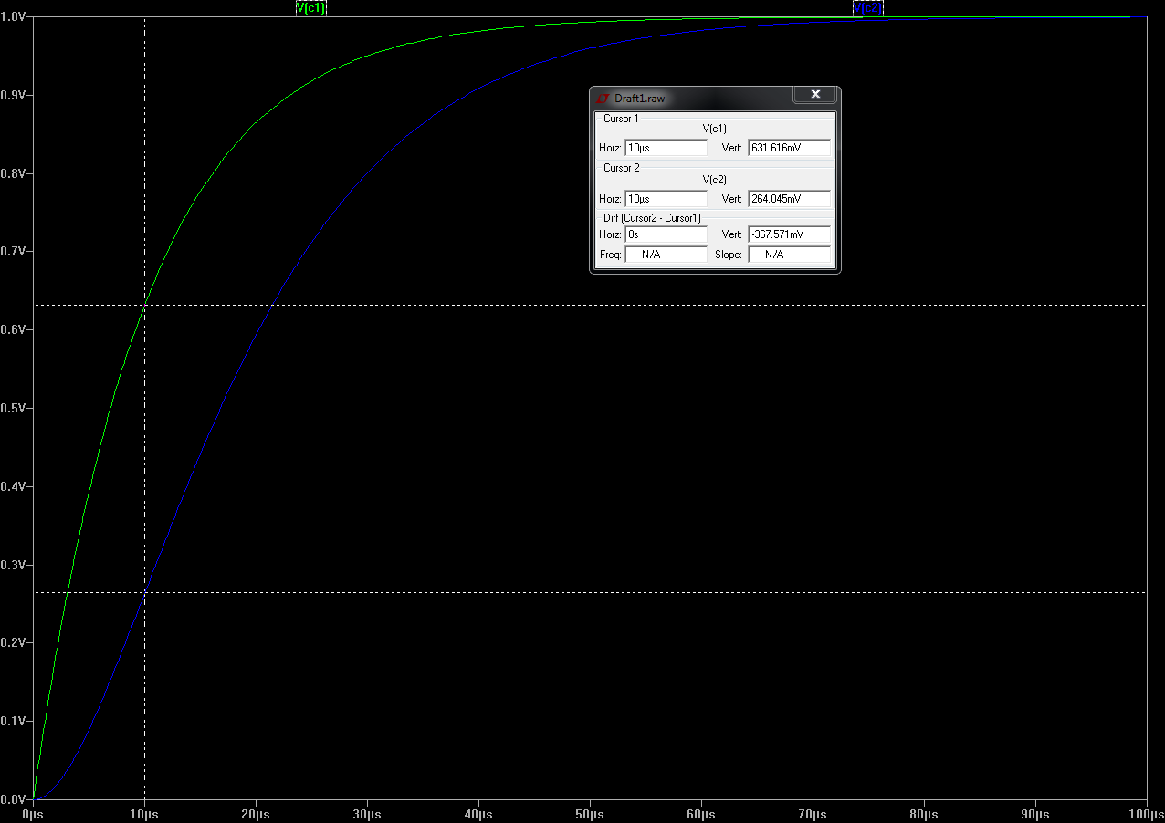
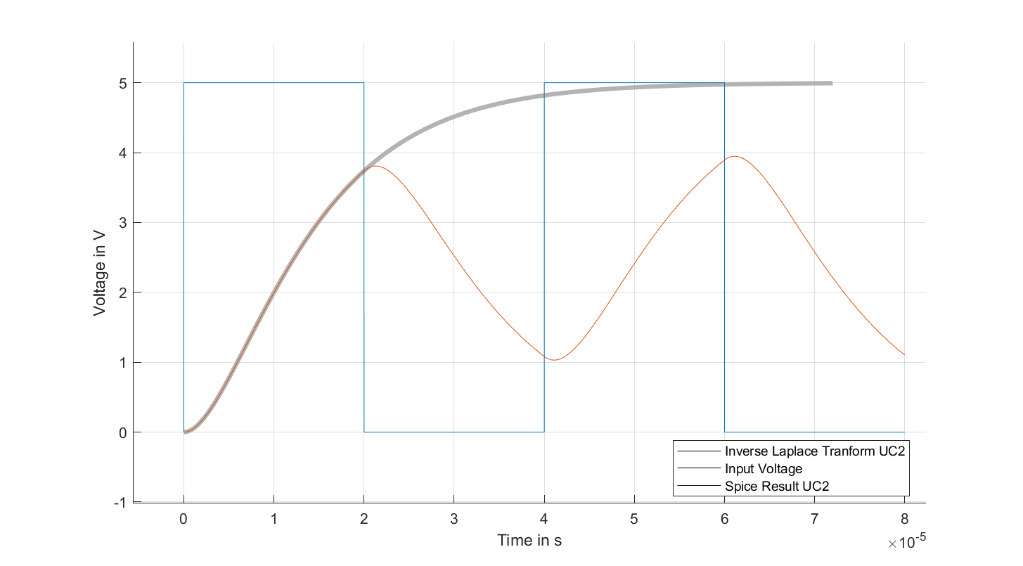
See attachment for a comparison with LTSpice. Legend colors are broken,
but I think you get the idea. Gray line is calculated with the formula
above, blue is input voltage and red is UC2, calculated by spice.
Obviously, only the first "active" period of the input signal is correct
here since I modeled an input step instead of a pulse.
Werner schrieb:> Die Schaltung existiert bereits und ich muss sie anwenden.
Oh, I thought it was a purely educational exercise on unit step
transient response. Why are you so concerned about initial voltages on
capacitors? If there's no supernatural mechanism, that's not shown on
the schematic, but somehow injecting charge to the capacitors, then
their voltages inevitably depend only on the input signal (i.e. you
can't realistically set them independently). What shape does your actual
input excitation have? Unit step? Infinite pulse train? Semi-infinite
pulse train, starting from t=0? Or ramp? Or some arbitrary shape? It's
hard to give meaningful advice without knowing these details.
LumpedNetwork schrieb:> Why are you so concerned about initial voltages on> capacitors?
My circuit is a feedback loop. A voltage is switched on (0 -> 5V) and
applied to a double RC network (PT2). When the output of the network
reaches a (user defined) threshold, the voltage is switched off again.
The switch off time is fixed. During that, the capacitors discharge. But
not completely! Consequently, in the next cycle the system has an
initial voltage which is not zero. By coincidence I can determine these
voltages.
For my task I need to know the "on" time. That is the time it takes to
charge the system until the threshold voltage is reached.
I didn't want the forum to solve my task. So I asked for education.
Would you say it is possible to solve my task, if I substitute one RC
network by an integrator? I would get rid of one exp() term and above
equation would be (algebraically) solveable, isn't it?
Trotz oder gerade wegen der spannenden Theorie hier würde ich jetzt für
den anstehenden konkreten Fall die Rechnung erst mal vernachlässigen! Du
weißt doch recht genau, dank Spice, wie die Spannungen aussehen und zwar
für den Zeit- und den Frequenzbereich. Wenn du da jetzt plötzlich einen
Integrator zu nimmst, veränderst du den Aufbau aber erheblich. Bleib
doch erst mal bei dem Aufbau jetzt. Im Übrigen habe ich jetzt dein
Problem mit dem zweiten RC-Glied nicht wirklich verstanden.
Offensichtlich kann die Eingangsspannung dort  beliebig zwischen 0 und
U(e) sein...ja und??? Das bedeutet doch nur, dass du mit der zweiten
Spannung mehr oder weniger schnell das Maximum erreichst. Ob das für
deine Regelung (?) nun relevant ist, kann man (ich) hier nicht sagen.
Bin aber gespannt, wie es weitergehen wird!
Gruß Rainer
Werner schrieb:> My circuit is a feedback loop.
OK, now I got it. So you're dealing with a steady state process. I don't
see a way to solve it generally. But if the poles are well split, I
would ignore the smaller time constant and solve it only for one
exponent. Whether this is satisfactory, depends on the particular values
of the elements and Toff.
Jan K. schrieb:> Strangely Heaviside was not taught in our classes and I can't find much> literature. Do you have some?
Most likely, it's not taught at all. The only article on this topic that
I know of is this one: https://ieeexplore.ieee.org/document/168699
(Supplementary paper:
https://www.ncbi.nlm.nih.gov/pmc/articles/PMC5832410/ )
The origins of the method are probably described in the book "E.Hallen
Tvungna svängningar operatorkalkyl, 1965", which I can't find anywhere,
unfortunately.